 Products Home / イメージングシステム&部品 / OCTイメージング(光干渉断層計)システム&コンポーネント / スペクトルドメインOCT(SD-OCT)システム Ganymede®シリーズ
スペクトルドメインOCT(SD-OCT)システム Ganymede®シリーズ

Please Wait
OCT製品の改良について
当社ではOCTベースユニットを改良し、新しく下記の機能を追加しました。
- より大きな実験装置への組み込みを可能にするトリガ設定
- OCT信号をほかのデータソースと結合するためのアナログ入力
- トラブルシューティング機能を改善する内部ハードウェア診断
SD-OCTシステム用高剛性(標準型)スキャナにおけるマイクロメータのネジ部の設計を刷新し、参照アームの位置決めをより精密に行えるようになりました。
ソフトウェアThorImage®OCTに、スペックル除去フィルタ、3次元スペックル分散モード、および自動ピーク検出の新機能が追加されました。
構成のオプション選択について

当社では、お客様のニーズに合わせたOCTシステムの構成をご提案いたします。試料をお送りいただければ、いくつかのオプション構成で取得した測定画像を
ご提供することも可能です。
また、オフィス併設のデモルームにてデモのご要望も承っております。詳しくは「OCTデモルーム」タブをご覧になるか、当社までお問い合わせください。
見積もり依頼について
OCTシステムの価格は構成部品によって
異なります。お客様のニーズに合ったシステムの構成に
ついては当社までご相談ください。
特注について
こちらをクリックすると当社の特注対応について
ご覧いただけます。

特長
- 構成をカスタマイズできる高分解能OCTシステム
- 中心波長が880 nmのスペクトルドメインOCTシステム(仕様については下表参照)
- 最高A-スキャンレート:248 kHz
- 最大イメージング深度(空気中):3.4 mm
- 軸方向分解能(空気中):< 3.0~6.0 µm
- 最高感度:106 dB
- PCおよびThorImage®OCTソフトウェアパッケージが付属
(「ソフトウェア」タブ参照) - 予め構成された基本構成システム、またはカスタム構成
基本構成システムの他、カスタム構成も可能
- 幅広い用途向けに最適化されたベースユニットから選択可能
- 走査システムとして、高剛性スキャナと調整機能付きスキャナをご用意
- USB 3.0またはCameraLink接続によるデータ取得
- 走査レンズキットは、横方向分解能および焦点距離を用途に合わせて最適化
- 試料用Zスペーサ(オプション)は、走査レンズ-試料間の媒質が空気または液体のイメージング用途に合わせ、リング型および液浸型をご用意
- その他、スキャナ用スタンドや移動ステージなどのアクセサリもご用意
- お見積りのご依頼やシステム構築、カスタマイズに関するご相談は当社 までご連絡ください。
光コヒーレンストモグラフィ(OCT)は、非侵襲な光学イメージング技術であり、試料の2次元断層画像および3次元ボリューム画像をリアルタイムで取得できます。この技術は、試料内の異なる層からの後方散乱光を用いて、試料の構造をµmレベルの分解能で数mmの深度まで画像化します。OCTイメージングは超音波イメージングと同様な画像取得法を光学的に実現したものと見ることができます。超音波イメージングと比較して浸透深度は浅くなりますが、高い分解能が得られるイメージング技術です。高分解能に加えて、非接触、非侵襲というOCTの特長は、生体組織、小動物や工業材料などのイメージングに適しています。
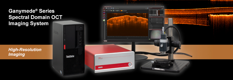
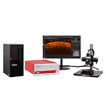
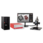
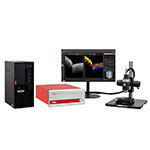
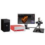
OCTイメージングシステムGanymede®シリーズは高分解能イメージング用として必要な柔軟性を備えており、Aスキャンの最高ライン速度は248 kHzです。付属のPCにプリインストールされている64ビットソフトウェアにより、2次元および3次元のOCTデータをリアルタイムで処理して表示します。カスタム構成の場合、スキャナは、堅牢な高剛性スキャナと調整機能付きスキャナからお選びいただけます。お客様の用途に合わせて、さらにOCTシステムをカスタマイズいただける、オプションのアクセサリもご用意しています(下記参照)。また、こちらのページでご紹介しているコンポーネントをベースにした組立て済みの880 nm OCTシステムを5種類ご用意しています。
下記のコンポーネントでお手持ちの当社製OCTシステムに機能を追加し、簡単にアップグレードすることも可能です。ほとんどのシステムはアップグレード可能ですが、お手持ちのシステムをご要望に沿った用途向けに最適化するためには、当社にご相談いただくことをお勧めいたします。
Figure 1.2の写真をクリックするか、Table 1.3内の製品名をクリックすると詳しい製品情報をご覧いただけます。
| Table 1.3 Ganymede Customization Options |
|---|
| OCT Base Unit (Computer Included) |
| Scanning System |
| Scan Lens Kit |
| Reference Length Adapter (For Standard Scanners Only) |
| Adjustable Scanner Stand |
| Translation Stage |
| Preconfigured Systems |
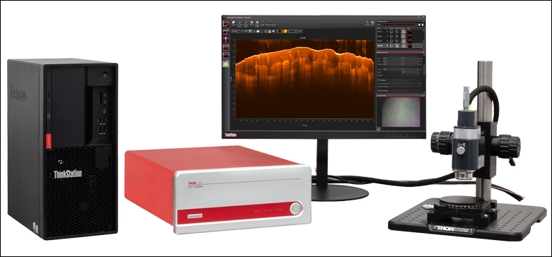
Figure 1.2 スペクトルドメインOCT(SD-OCT)システム Ganymedeシリーズ

ThorImage®OCT Software
Software features:
- Live Acquisition and Simultaneous Display in 1D, 2D, and 3D
- Live Sample Monitor for Easy Sample Positioning and Adjustment of Scan Pattern
- Advanced Dataset Handling
- User Access from Calibration and Raw Data Through to Processed Data
- Various Data Export Options
- Time-Series Measurements
- Doppler, Speckle Variance, and Polarization-Sensitive (PS)a Acquisition Modes
- Lightweight API ThorImageAutomation (C, C#, LabVIEW and Python)
- Low-Level SDK APIs Available In C, LabVIEW, and Python
- Seamless Integration of User-implemented Python Processing in ThorImageOCT Environment
ThorImage®OCT is a high-performance data acquisition software that is included with all Thorlabs OCT systems. This 64-bit Windows-based software acquires and displays OCT data and includes scan control and processing options. Additionally, Python, NI LabVIEW®, and C-based Software Development Kits (SDKs) are available, which contain a complete set of libraries for measurement control, data acquisition, and processing, as well as for storage and display of OCT images. The SDKs provide the means for developing highly specialized OCT imaging software for any individual application. The Python user interface enables user-developed processing routines within the ThorImageOCT live view.
| Table 116B ThorImageOCT Documentation | |
|---|---|
| ThorImageOCT Software Manual | |
| Third-Party Software License Agreements | |
Video 116A shows OCT images of a finger being acquired and manipulated in ThorImageOCT. This is done using the 3D volume and cross section modes. The software manual and third-party license agreements are included in Table 116B.
Explore the functionality of the ThorImageOCT software by clicking the expandable Workspace, Capabilities, Feature Plugins, Integration, and Specifications bars below. See the Specifications bar for a complete list of features and compatibility.
- Specific PS system required.
Workspace
ThorImageOCT streamlines the image acquisition and analysis process with a user-intuitive, feature-rich workflow. Control panels are designed so that the most important features are readily available and users can quickly set up their experiment. Panel layouts are completely customizable for different use cases or imaging modalities. All software features are easily accessible from the main workspace window, providing a complete, self-contained software package.
Click the Highlighted Regions in Figure 116C to Explore the Workspace

Figure 116C ThorImageOCT Workspace Window
Capabilities
| Quick Links |
|---|
| Acquisition |
| Imaging Modes: 1D, 2D, and 3D Scan Control with Sample Monitor Probe Calibration Image Quality and Speed |
| Processing |
| Image Field Correction |
| Image Viewing |
| Viewing Options Dataset Management |
| Analysis |
| Despeckle Filter Marker Tool Surface Detection |
Acquisition
Imaging Modes
Different OCT imaging modes can be selected using the mode selector. If the ThorImageOCT software finds a compatible system connected and switched on, all operational modes will be selectable. If no OCT device is present, only the data viewing mode for viewing and OCT data export will be available.
Click to Enlarge
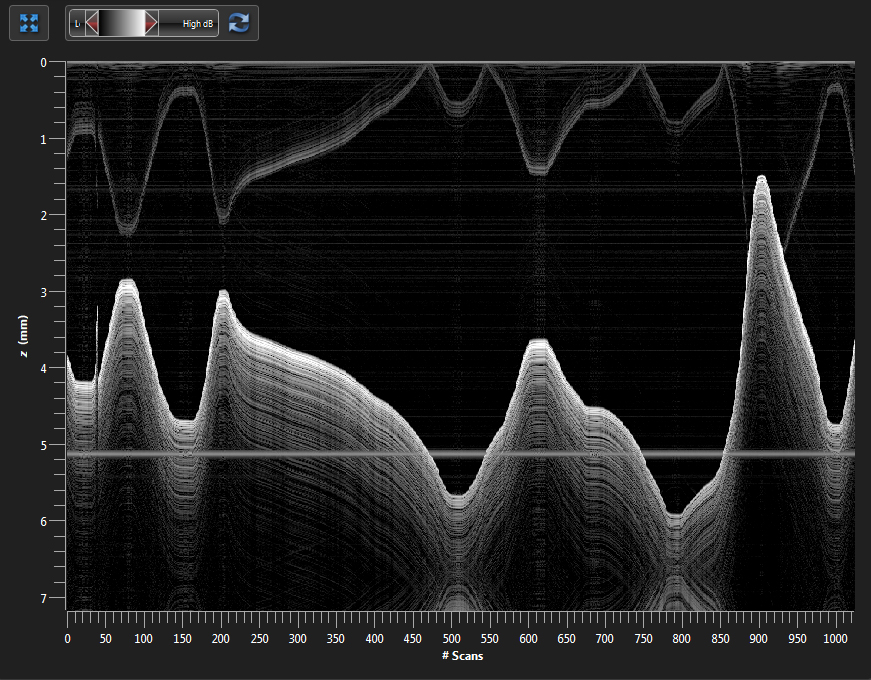
Figure 116E Several A-Scans at a Single Point Over Time (M-Scan)
Click to Enlarge
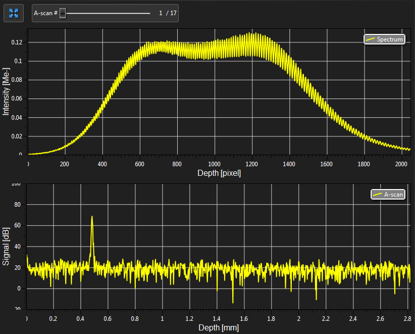
Figure 116D Spectral and Depth Information for a Single Point (A-Scan)
1D Mode
In this mode, single-point measurements can be made that provide spectral and depth information, as well as the ability to observe time-related sample behavior with an M-scan.

Click to Enlarge
Figure 116F ThorImageOCT Window in the 2D Mode
2D Mode
In the 2D imaging mode, the probe beam scans in one direction, acquiring cross-sectional OCT images that are then displayed in real time. Acquisitions can be stored with Snapshot and Advanced Snapshot. Advanced Snapshot provides optimized averaging options for higher image quality. For long term measurements, a time series function with an adjustable time interval between two acquisitions is included. Image display parameters, such as color mapping, can be controlled in this mode. We have also implemented an option for automatic calculation of the optimum contrast and brightness of the displayed OCT images.
Click to Enlarge
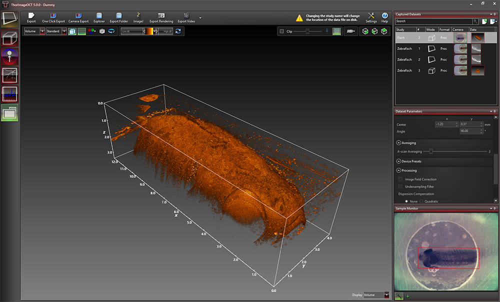
Figure 116G Rendering View in ThorImageOCT
3D Mode
In the 3D imaging mode, the OCT probe beam scans sequentially across the sample to collect a series of 2D cross-sectional images that are then processed to build a 3D image.
Utilizing the full potential of our high-performance software in combination with our high-speed OCT systems, we have included a Fast Volume Rendering Mode in the ThorImageOCT software, which serves as a preview for high-resolution 3D acquisitions. In this mode, high-speed volume renderings can be displayed in real-time, providing rapid visualization of samples in three dimensions.
To accommodate long term measurements, a time series function that takes a series of 3D measurements is available. The number of volumes to be acquired and the time interval between scans are adjustable.
Click to Enlarge
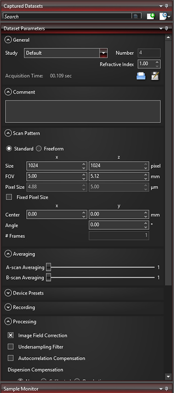
Figure 116H Various acquisition parameters can be adjusted in ThorImageOCT.
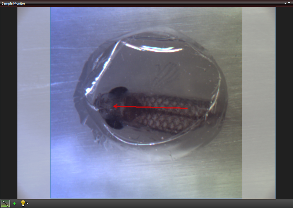
Scan Control with Sample Monitor
ThorImageOCT provides numerous scan and acquisition controls. The camera integrated in the scanner of our OCT systems provides live video images in the application software. Defining the scan line for 2D imaging or the scan area for 3D imaging is accomplished through the easy-to-use "Draw and Scan" feature by clicking on the video image.
Click to Enlarge
Figure 116J The Sample Monitor can be used to define the scan pattern using the "Draw and Scan" feature.
Arbitrary forms defined by the Draw & Scan feature or loaded .txt files can be scanned. The scan pattern can also be adjusted by specifying suitable parameters in the controls of the software, as shown in Figure 116H.
Click to Enlarge
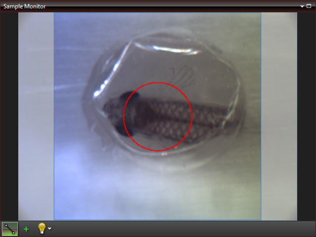
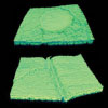
Figure 116K A predefined circle scan pattern can be loaded and scanned in the software. The size can be changed with the Zoom feature.

Click to Enlarge
Figure 116L A predefined triangle scan pattern can be loaded and scanned in the software. The size can be changed with the Zoom feature.
Additionally, one can further set processing parameters, averaging parameters, and the speed and sensitivity of the device using device presets. By using a high-speed preset, video-like frame rates in 2D and fast volume rendering in 3D are possible, whereas high-sensitivity acquisition is enabled by choosing a preset with a lower acquisition speed.
Click to Enlarge
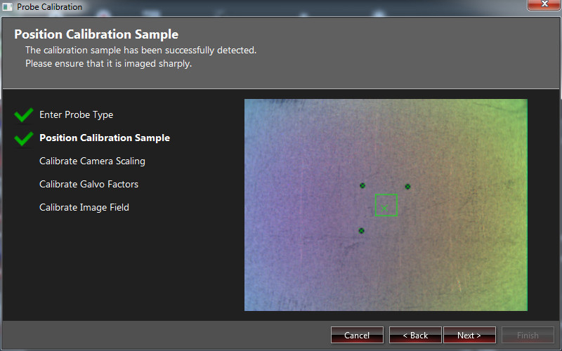
Figure 116M Probe Calibration Window in ThorImageOCT
Probe Calibration
Our camera and scanning system are calibrated to match the real lengths for the scan pattern parameter. Changing to a different scan lens kit will generally require a different probe configuration in order to adapt to changes in the optical parameters of the system. When an additional scan lens is purchased for your Thorlabs OCT scanner system, ThorImageOCT enables you to easily create a fitting configuration for your new scan lens by using the calibration sample shipped with the lens and an intuitive step-by-step calibration process (shown in Figure 116M).
Image Quality and Speed
Depending on the specific application, the balance between image quality and acquisition time may tend more towards one or the other. Several options based on the available hardware are provided to help reach the optimal balance for a given measurement.
Averaging
Averaging the spectra before the Fast Fourier Transform (FFT), or averaging the processed data with A-Scan averaging or B-scan averaging are two options available that can enhance the image quality or the acquisition speed.
Speed and Sensitivity
For camera based systems of the Ganymede and Telesto family, predefined presets of the acquistion speed can be chosen. By using a high-speed preset, video-live frame rates in 2D and fast volume rendering in 3D are possible, whereas high-sensitivity acquistion is enabled by choosing a preset with a lower acquistion speed.
Additional Controls
For the Vega and Atria System families, the Detector Gain is adjustable in ThorImageOCT. Additional controls to match the polarization state of the light from the sample and reference arm as well as a software integrated reference stage to adjust optical length of the reference arm are included.
Processing
ThorImageOCT provides features specifically designed to improve the quality of OCT images. The data can be modified during acquisition using processing parameters, such as image field correction, dispersion correction, and undersampling filters, or afterwards with filters.
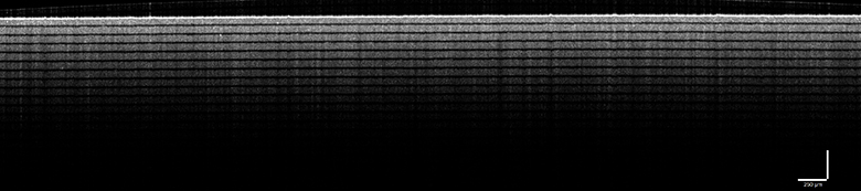
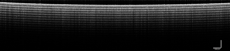
Image Field Correction
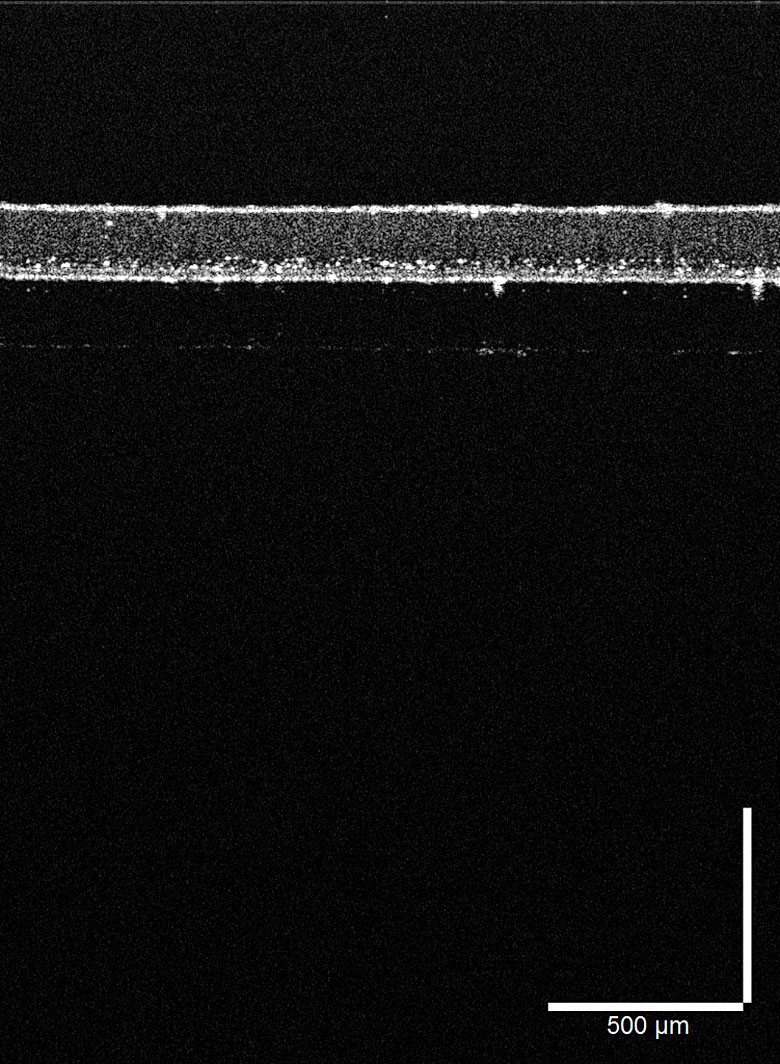
A calibrated image field correction is included by default with the system. This corrects optical distortions in the axial direction and is demonstrated on scotch tape in Figure 116N and Figure 116P.
Click to Enlarge
Figure 116P Image Field Correction Applied to an OCT Image of Scotch Tape
Click to Enlarge
Figure 116N OCT Image of Scotch Tape
If additional processing functions are desired, ThorImageOCT can also integrate user-defined processing and post-processing algorithms; see the External Programs and User Interface for Python Processing sections in the Integration tab below for more details.
Image Viewing
For all imaging modes, an offline mode is available to view acquired images with ThorImageOCT stored as .oct-files. All legacy .oct-files can be opened with the current version of ThorImageOCT.
Viewing Options
In the ThorImageOCT software, 3D volume datasets can be viewed as orthogonal cross-sectional planes (see Figures 116Q and 116R) and volume renderings. The Sectional View features cross-sectional images in all three orthogonal planes, independent of the orientation in which the data was acquired. The view can be rotated as well as zoomed in and out.
The Rendering View provides a volumetric rendering of the acquired volume dataset. This view enables quick 3D visualization of the sample being imaged. Clip planes of any orientation can be applied. The 3D image can be zoomed in and out as well as rotated. Furthermore, the coloring and dynamic range settings can be adjusted.
Click to Enlarge
Figure 116Q Sectional View in ThorImageOCT
Click to Enlarge
Figure 116R Rendering View in ThorImageOCT
Click to Enlarge
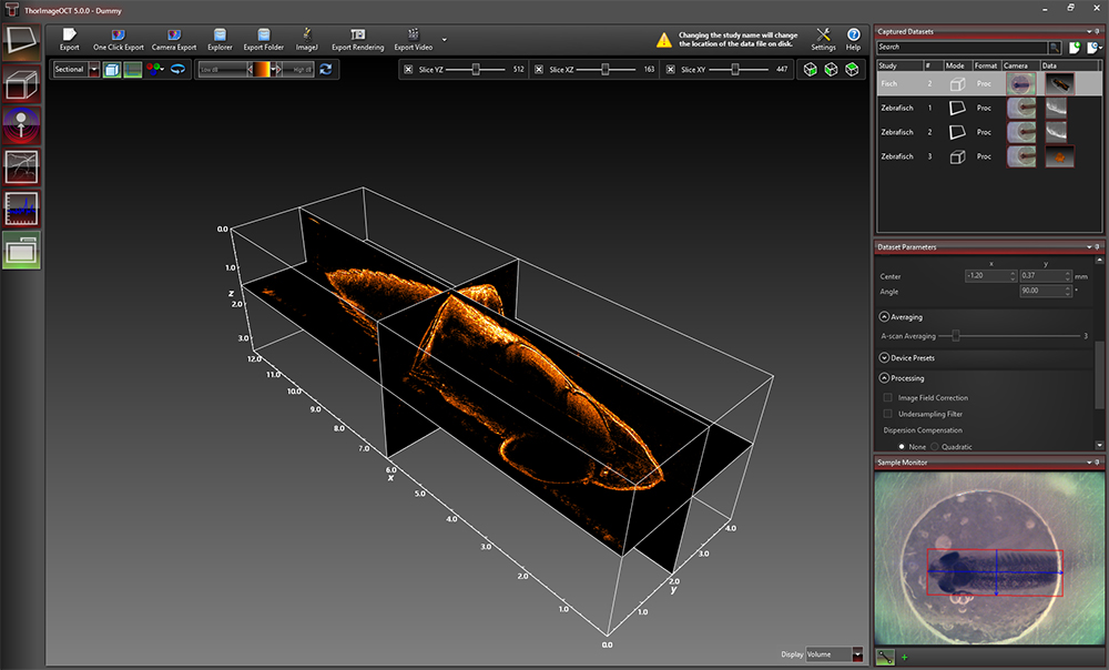
Figure 116T The Dataset Management Window of ThorImageOCT
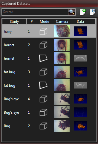
Dataset Management
ThorImageOCT provides advanced dataset management capabilities, which allow several datasets to be opened simultaneously. Datasets are uniquely defined using an identifier consisting of a study (or test series) name and an experiment number. Grouping of datasets can be achieved by using the same study name. The "Captured Datasets" list shows an overview of all open datasets, including the dataset identifier, the acquisition mode, and preview pictures of the still video image and the OCT data.
.oct Files and Export
The OCT file format native to ThorImageOCT allows OCT data, sample monitor data, and all relevant metadata to be stored in a single file. ThorImageOCT can also be installed and run on computers without OCT devices in order to view and export OCT data. The user has full access to the raw and processed data from the device, including additional data used for processing, e.g. offset errors.
Datasets can be exported in various image formats, such as PNG, BMP, JPEG, PDF, or TIFF. The set can also be exported in complete data formats suited for post-processing purposes, such as RAW/SRM, FITS, VTK, VFF, and 32-bit floating-point TIFF.
Click to Enlarge
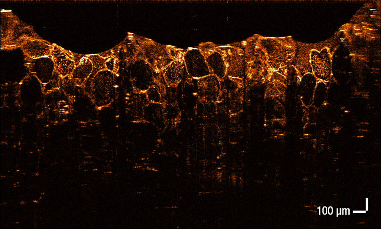
Figure 116V Despeckle Filter Applied to an OCT Image of a Human Tooth

Click to Enlarge
Figure 116U OCT Image of a Human Tooth
Analysis
ThorImageOCT includes several tools for convenient data analysis. The integrated marker tool measures distances, as well as the structure size. Additionally, this tool can be used to display the intensity profile of the OCT data across a line. For precise distance and thickness measurements, the refractive index of the material under investigation can be set.
Despeckle Filter
The Despeckle Filter is an optimized image filter to reduce speckle noise without blurring details of the imaged structure. It can be turned on and off for all acquired 2D images in the offline mode.
As shown in Figure 116V, the despeckle filter can be applied to an image to reduce speckle noise without blurring details of the imaged structure.

Click to Enlarge
Figure 116X The marker tool can be used to measure layer thickness.
Click to Enlarge
Figure 116W Surface Detection Tool
Marker Tool
The integrated marker tool serves to measures distances, as well as the structure size. Additionally, this tool can be used to display intensity profile of the OCT data across a line. For precise distance and thickness measurements, the refractive index of the material under investigation can be set.
Surface Detection
The Surface View performs a segmentation of the outer surface of the object viewed in the OCT section. The surface is then rendered with colors indicating the actual depth and can be filtered to reduce the effect of noise.
Feature Plugins
| Quick Links |
|---|
| Doppler Mode Speckle Variance Mode Polarization-Sensitive Modes Python User Interface for Processing |
Click to Enlarge
Figure 116Y Doppler Dataset Showing the Velocity of a Rotated Plastic Stick with Opposite Flow Directions.
Doppler Mode
Doppler OCT imaging comes standard with all OCT systems. In the Doppler mode, phase shifts between adjacent A-scans are averaged to calculate the Doppler frequency shift induced by particle motion or flow. The number of lateral and axial pixels can be modified to change velocity sensitivity and resolution during phase shift calculation. The Doppler images are displayed in the main window with a color map indicating forward- or backward-directed flow, relative to the OCT beam.
Click to Enlarge
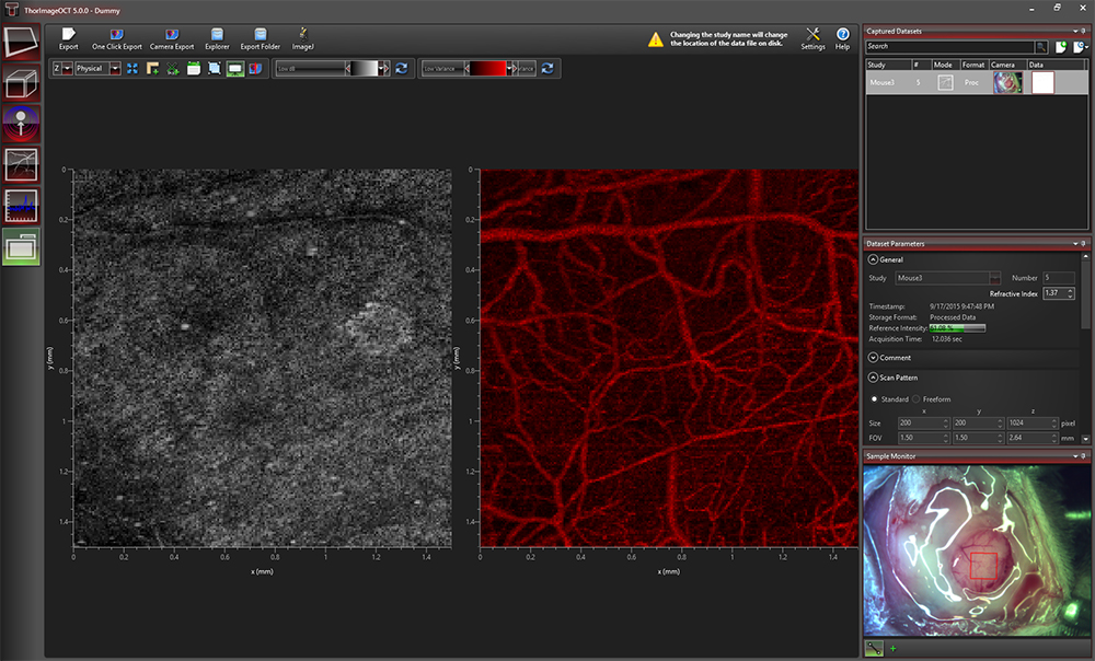
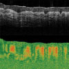
Figure 116Z Speckle Variance Measurement Showing Blood Vessels of a Mouse Brain.
Speckle Variance Mode
The speckle variance imaging mode is an acquisition mode that uses the variance of speckle noise to calculate angiographic images. It can be used to visualize three dimensional vessel trees without requiring significant blood flow and without requiring a specific acquisition speed window. The speckle variance data can be overlaid on top of intensity pictures providing morphological information. Different color maps can be used to display the multimodal pictures.
Polarization Sensitive
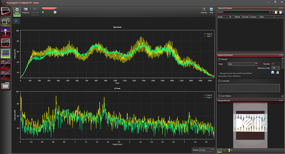
In the Polarization-Sensitive OCT (PS-OCT) system, two additional imaging modes are available, and the 1D mode is augmented to show each camera's spectra simultaneously. The combination of both cameras, and therefore the unique additional information of the PS-OCT system, is implemented in the 2D and 3D Polarization-Sensitive Imaging Modes.
Click to Enlarge
Figure 116AA Several A-Scans at a Single Point Over Time (M-Scan)
1D Mode
In this mode, single-point measurements can be made that provide spectral and depth information, as well as the ability to observe time-related sample behavior with an M-scan. For single-point measurements, the simultaneously acquired spectra of the two line scan cameras in the PS-OCT system are displayed separately.
Click to Enlarge
Figure 116AB Spectral and Depth Information for a Single Point (A-Scan)
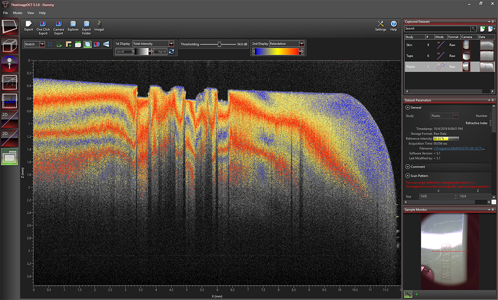
2D Polarization-Sensitive Mode
The 2D polarization-sensitive imaging mode acquires cross-sectional OCT images and displays them in real time. It has two configurable displays, each able to show one of the following images: a single camera's intensity, a combination of both cameras' intensities, or polarization data such as retardation, optic axis, DOPU or a single Stokes parameter. To improve the image quality or allow for variable acquisition time, several averaging parameters and adjustable line rates are implemented. Image display parameters, such as color mapping or thresholding, can be controlled in this mode. We have also implemented an option for automatic calculation of the optimum contrast, brightness, and thresholding of the displayed OCT images that operates on the intensity and PS-OCT images.
Click to Enlarge
Figure 116AC ThorImageOCT Window in 2D Polarization-Sensitive Mode

Click to Enlarge
Figure 116AD Dual Display Configuration of 2D Polarization-Sensitive Mode

Click to Enlarge
Figure 116AE The ThorImageOCT window in the 3D Polarization-Sensitive Mode
3D Polarization-Sensitive Mode
The 3D polarization-sensitive imaging mode extends the 3D imaging mode. The acquisition and display options are the same as in the 3D imaging mode. Additionally, the user can choose to display one of the following rendered volume imaging options: an intensity OCT image (from either a single camera or the combination of both) or a PS-OCT image (such as retardation, optic axis, DOPU or one of the three Stokes parameters). The rendered PS-OCT images can be adjusted with a threshold computed out of the intensity OCT image to only display the polarization-sensitive data of regions above the noise.
ThorImage OCT includes a Fast Volume Rendering mode, which provides a preview for high-resolution 3D acquisitions of intensity and PS-OCT images. In this mode, high-speed volume renderings can be displayed in real time, providing rapid visualization of samples in three dimensions.

Click to Enlarge
Figure 116AF Dataflow with Python Processing
Python User Interface for Processing
The Python Processing feature enables the advanced user to bypass the default signal processing routines and seamlessly integrate experimental/prototypical signal processing algorithms directly into the ThorImage environment. This provides utility both in the research (development of signal processing and analysis routines) and educational domains. Key features include:
- Write Customized Signal Processing Routines Using Python Syntax
- Utilize the Wide Array of Python Open-Source Signal Processing, Image Analysis, and Machine Learning Libraries
- Parameterize Algorithms and Routines
- Python Outputs and Debugging Messages Print Directly in ThorImage OCT
- Display Plots and Visualize Processing Steps with The Matplotlib Library
- Demo Implementations and Code Documentation Included
- Supports 1D, 2D, and 3D Imaging Modes of all Thorlabs OCT Systems (Excepting Doppler, Speckle Variance, and Polarization-Sensitive Imaging Modes)
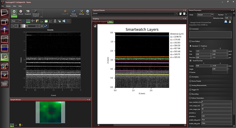
Layer Thickness Measurement
The Python Processing Interface also allows users to integrate customized post-processing algorithms for data modification or analysis. The demo program, shown in Figure 116AG, displays an OCT scan of the inner layers of a smart watch. By extending the signal processing algorithms with appropriate segmentation methods, the python processing feature can be used to highlight the individual layers and compute the distances in between.
Click to Enlarge
Figure 116AG Python Demo Program Post Processing Thickness Layer Measurement of a Smart Watch
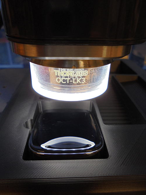
Click to Enlarge
Figure 116AH Smartwatch Under OCTG13 with OCT-LK3
Integration
| Quick Links |
|---|
| Data Export Hardware Synchronization Third-Party Integration Software Development Kits Custom Programming Options User Guide |
Data Export
Datasets can be exported in various image formats, such as PNG, BMP, JPEG, PDF, or TIFF. The set can also be exported in complete data formats suited for post-processing purposes, such as RAW/SRM, FITS, VTK, VFF, and 32-bit floating-point TIFF.
The OCT file format native to ThorImageOCT allows OCT data, sample monitor data, and all relevant metadata to be stored in a single file. ThorImageOCT can also be installed and run on computers without OCT devices in order to view and export OCT data. The user has full access to the raw and processed data from the device, including additional data used for processing, e.g. offset errors.
Click to Enlarge
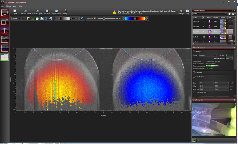
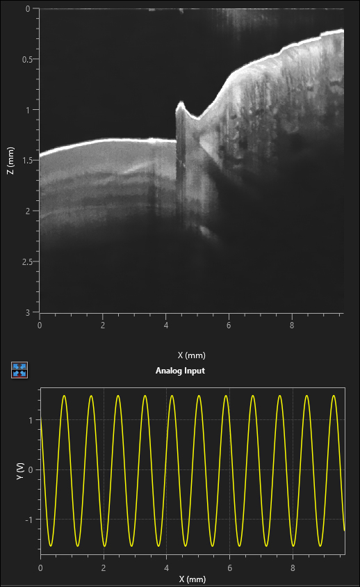
Figure 116AJ Analog Data Visualization in the 2D Display
Hardware Synchronization
Externally-Triggered Acquisition
ThorImageOCT and the SDK APIs (in C, LabVIEW, and Python) provide the ability to externally trigger the acquisition of A-Scans. This enables the user to synchronize measurements from different modalities (e.g. vibrometry and synchronized positioning) with an OCT measurement. Synchronization is greatly simplified with all current CameraLink-based Thorlabs OCT systems (a TTL level trigger signal source is required). External triggering is available for all imaging modes and can be toggled in the settings dialog in ThorImageOCT.
Thorlabs' current generation of Ganymede and Telesto SD-OCT, and the Telesto PS-OCT Systems include an external B-Scan trigger for synchronization with other experiments.
Analog Input for Synchronization with Other Modalities
Thorlabs' current generation of Ganymede and Telesto SD-OCT, and the Telesto PS-OCT Systems include two analog input channels, which can be used to combine imaging modalities. The analog signal from another data source (i.e., fluorescence signal) is sampled and displayed simultaneously with the OCT signal.
Third-Party Integration

Click to Enlarge
Figure 116AK Export buttons are accessible in the Action Toolbar of ThorImageOCT.
Link to ImageJ
If both ImageJ and ThorImageOCT are installed on the computer, opening acquired OCT data in ImageJ is one mouse click away. This enables a smooth workflow when requiring the advanced image processing functionality provided by ImageJ. Clicking the Explorer button will open the folder and select the file in Windows Explorer where the currently active dataset is stored.
External Program
Click to Enlarge
Figure 116AN After smoothing the data in ImageJ, the marker tool in ThorImageOCT can be used to measure layer thickness.

Click to Enlarge
Figure 116AM A filter for smoothing lateral directions is applied to the image in ImageJ.
Click to Enlarge
Figure 116AL OCT Data of a Plastic Multilayered Film with Speckle
Acquired OCT datasets can also be exported and modified in a third-party program, and then reimported back into the ThorImageOCT software. This functionality allows fast and customized modifications of OCT images, while still using the dataset management of the ThorImageOCT software. As shown in Figures 116AL, 116AM, and 116AN, OCT data (Figure 116AL) can be exported to ImageJ and a smoothing filter applied in the lateral direction (Figure 116AM). Using the "External Program" button allows the modified data to be reimported into ThorImageOCT for further analysis. For example, the peak detection tool can be used to measure the layer thicknesses (Figure 116AN).
Python User Interface for Processing
The Python User Interface for Processing described in the Feature Plugins tab above enables user-development of customized processing routines, and allows for live display of these processing routines.
Click to Enlarge
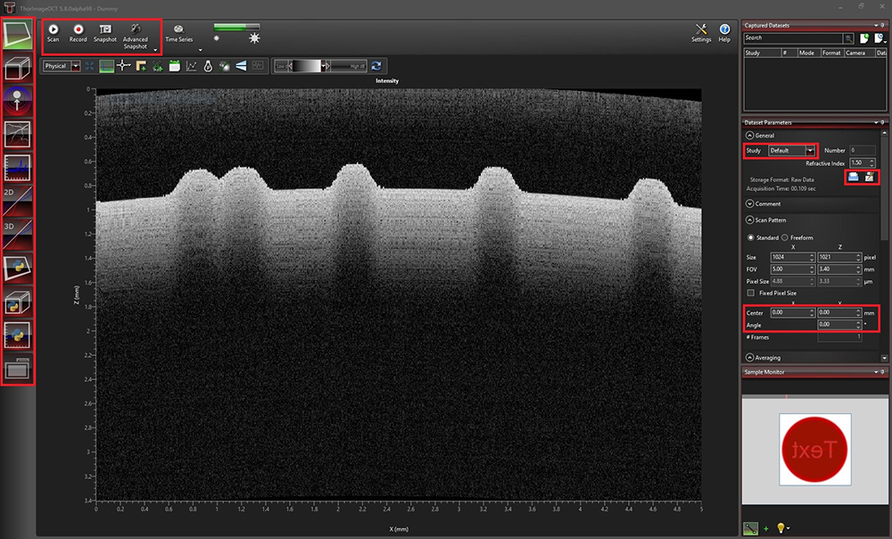
Figure 116AP Available ThorImage Automation Functions Marked in Red from ThorImageOCT GUI in the 2D Acquisition Mode
Software Development Kits
Spectral Radar APIs
For maximum flexibility, customized solutions can be implemented in ThorImageOCT using software development kits (SDKs). Experienced software developers can use these in a multitude of programming environments to tailor the use of Thorlabs OCT systems to their specific application. SDKs are available in:
- ANSI C
- LabVIEW®
- Python
ThorImage Automation
ThorImage Automation is a light-weight API for performing OCT tasks through the ThorImageOCT GUI. This is in contrast to the SpectralRadar API, which communicates directly with the device. SpectralRadar offers large flexibility, whereas ThorImage Automation enables implementation of simple OCT task with a minimal amount of code.
ThorImage Automation is available in:
- C
- C#
- LabVIEW
- Python
Custom Programming Options User Guide
Table 116AQ provides guidance on choosing the right programming option for the user depending on the user requirements, programming experience and capabilities of the software.
| Table 116AQ ThorImage®OCT Programming Options User Guide | |||||
|---|---|---|---|---|---|
| SDK APIs | ThorImage Automation | Python Processing | External Program | ||
| Entry Point | User Program | User Program | ThorImageOCT GUI | ThorImageOCT GUI | |
| Flexibility/Limitation | Great Flexibility | Limited to Specific ThorImageOCT GUI Functionality | Limited to OCT Processing Functionality | Limited to OCT Post Processing Functionality | |
| Programming Level | Low Level | High Level with Very Little Code | Low Level (OCT Processing Only) | Low-Medium Level (Post Processing Only) | |
| Online/Offline | Full Control on User Side | Online (Hook to Specific ThorImageOCT GUI Functions to the Code) | Online (User Processing Code Used in ThorImageOCT GUI) | Offline (Feature in ThorImageOCT GUI) | |
| ThorImageOCT Running/Usable At the Same Time | No | Yes | Yes | Yes | |
| Software | C | Yes | Yes | No | Arbitrary Third-Party Software |
| C# | Via C-API | Yes | No | Arbitrary Third-Party Software | |
| LabVIEW | Yes | Yes | No | Arbitrary Third-Party Software | |
| Python | Yes | Yes | Yes | Arbitrary Third-Party Software | |
| Example User REquirements: Implementation of ... | User GUI | Yes | No | No | No |
| User OCT Processing | Yes | No | Yes | No | |
| User Post Processing | Yes | No | No | Yes | |
| Automation | Yes | Yes | No | No | |
| Recommended OCT Knowledge | Advanced | Beginner | Beginner | Beginner | |
| Rocommended OCT Processing Knowledge | Beginner | Beginner | Advanced | Beginner | |
Specifications
| ThorImage®OCT Specifications | ||
|---|---|---|
| General | Compatibility | |
| OCT Method |
| |
| Imaging Modes |
| |
| Operating System |
| |
| Acquisition | Synchronization Options |
|
| Sample Monitor |
| |
| Data Acquisition |
| |
| Speed/Sensitivity |
| |
| Scan Control |
| |
| Averaging |
| |
| Apodization |
| |
| Probe Calibration |
| |
| Processing | GUI |
|
| Python Processing Interface |
| |
| Data Viewing | Common Options |
|
| 2D Mode |
| |
| 3D Mode |
| |
| Analysis | Native Tools |
|
| Third-Party Integration |
| |
| File Handling | .oct Files | Full Access To:
|
| File Export |
| |
| SDKs | Spectral Radar API |
|
| ThorImageAutomation |
| |
| Settings | Workspace |
|
| Support | Technical Support |
|

For information on the availability of ThorImageOCT version 5.8, please contact our OCT Support Team.
OCTチュートリアル
光コヒーレンストモグラフィ(OCT)は非侵襲の光学イメージング法であり、数mmの深さまでの1次元情報(深さ方向)、2次元の断層画像、および3次元のボリューム画像を、µmレベルの深さ分解能で、かつリアルタイムで取得することができます。OCTは試料内の各層からの後方散乱光を用いて、試料の構造情報を画像化します。OCTはリアルタイムで画像を取得できますが、さらに複屈折性を利用したコントラストの改善や、オプションの拡張技術を追加することで血流の機能的画像の取得も可能です。
当社では、簡単に持ち運べるコンパクト性を維持しながら、複数の波長、画像分解能、取得速度に対応した、様々なOCTイメージングシステム開発してきました。また、お客様固有のご要望にお応えするOCTイメージングシステムをご提供できるように、様々な用途に対して最適化できる、高度にモジュール化した製品の設計を進めてきました。
用途例
芸術作品の保存
薬剤皮膜
3次元プロファイリング
In Vivo
小動物
生物学
生体組織の複屈折
マウスの肺
網膜錐体細胞
Click to Enlarge
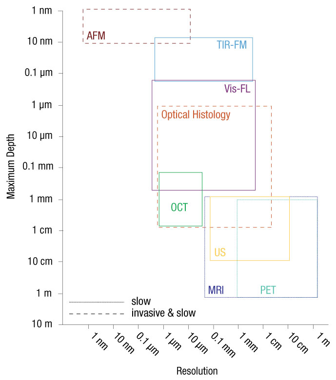
Figure 91A 様々なイメージング法における浸透深さと分解能
Click to Enlarge
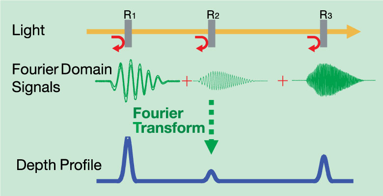
Figure 91B フーリエドメインOCTでは、遅延した参照ビームと試料からの後方散乱光の干渉によって生じるフーリエドメイン信号を解析することで、深さ方向のプロファイルを生成します。
OCTイメージングは超音波測定と類似する点がありますが、測定深度が浅くなる代わりに、非常に高い分解能が得られることが特長です(Figure 91A参照)。最大15 mmのイメージング範囲、軸方向分解能5 μm以上での画像化が可能なことにより、OCTは「超音波」測定と「共焦点顕微鏡」による測定とのちょうど中間の測定装置として位置づけられます。
高分解能で深部イメージングができるという特長に加えて、OCTには非接触、非侵襲という利点もあるため、生体組織や小動物、あるいは材料といった試料の画像取得に適しています。最近、OCT分野ではフーリエドメイン OCTと呼ばれる新しい技術が開発され、1秒間に700,000ライン以上の高速イメージングが可能になっています。1
フーリエドメイン光コヒーレンストモグラフィ(FD-OCT、Figure 91B参照)は、光源の干渉特性を利用してサンプル中での光路長遅延を測定する、低コヒーレンス干渉法に基づいています。OCTの干渉計は、 μmレベルの分解能で断層画像を得るために、サンプルから反射光と参照アームからの反射光の光路長の差を測定するように設定されています。
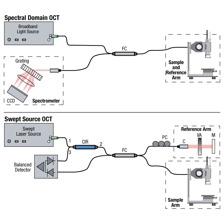
FD-OCTシステムは、光源と検出方式の違いによって、スペクトルドメイン OCT(SD-OCT)と波長掃引OCT(SS-OCT)の2つに分類されます。Figure 91Dに示すように、いずれのシステムでも光は干渉計のサンプルアームと参照アームに分割されます。SS-OCTシステムでは狭帯域幅のコヒーレンス光を利用し、SD-OCTシステムでは広帯域幅の低コヒーレンス光を利用します。サンプル中の屈折率の変化によって生じた後方散乱光は、サンプルアーム光路のファイバに再度結合し、さらに参照アームの固定された光路長を伝搬してきた光と重ね合わされます。その結果として得られるインターフェログラム(干渉パターン)は、干渉計の検出アームを通して測定されます。
光検出器によって測定されるインターフェログラムの周波数は、サンプル中での反射体の位置の深さに関係します。そのため、測定されたインターフェログラムをフーリエ変換することで、深さ(1次元)方向の反射率プロファイル(A-スキャン)が得られます。 サンプルアームのビームでサンプルを横断して走査すると、一連のA-スキャン情報を収集することができ、2次元断層画像(B-スキャン)が得られます。
同様に、OCTのビームを別の方向にも走査すると、連続した2次元画像を収集することができ、一組の3次元体積データが得られます。FD-OCTを用いると、2次元画像はミリ秒程度で得られ、3次元画像でも現在では1秒以下で得られます。
スペクトルドメインOCT(SD-OCT)と波長掃引OCT(SS-OCT)
SD-OCTと SS-OCTは同じ基本原理に基づいていますが、OCTのインターフェログラム生成の技術的アプローチが異なっています。SD-OCTは可動部を持たないために機械的な安定性に優れており、位相雑音が低くなります。幅広い種類のラインカメラが利用できるため、様々な画像取得速度や感度を有するSD-OCTシステムの開発が可能です。
SS-OCTシステムでは、周波数掃引光源とフォトディテクタを用いて、同様のインターフェログラムを高速で生成します。レーザ光源の波長掃引が高速なため、各波長で高いピークパワーの光をサンプルに照射することができ、光損傷のリスクをほとんど伴わずに感度を高めることができます。
Click to Enlarge
Figure 91D スペクトルドメインOCTシステムと波長掃引OCTシステムの比較
フーリエドメイン OCTの信号処理プロセス
フーリエドメインOCTでは、インターフェログラムは光周波数の関数として検出されます。参照アーム内の光遅延は固定されているため、サンプルの異なる深さからの反射光により異なる周波数成分の干渉パターンが生成されます。そして、フーリエ変換により異なる深さからの反射信号を分離する事で、サンプルの深さ方向プロファイルを得ることができます(A スキャン)。
1V.Jayaraman, J. Jiang, H.Li, P. Heim, G. Cole, B. Potsaid, J. Fujimoto, and A. Cable, "OCT Imaging up to 760 kHz Axial Scan Rate Using Single-Mode 1310 nm MEMs-Tunable VCSELs with 100 nm Tuning Range," CLEO 2011 - Laser Applications to Photonic Applications, paper PDPB2 (2011).
カタログとシステム構成図
下のボタンから印刷可能なPDF形式のカタログ、およびGanymede®シリーズOCTシステムのカスタマイズガイドがご覧いただけます。


Click to Enlarge
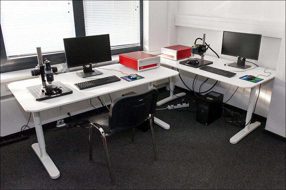
Figure 90A デモルーム例(ドイツオフィス)
OCTイメージングシステム:デモルーム・オンラインデモのご案内
ソーラボのアプリケーションスペシャリストや技術者は、日本やOCTシステムの製造施設があるドイツを始め、世界各地でお客様の実験用途に適したOCTシステムをお選びいただくためのお手伝いをいたします。当社では、お客様のニーズに合わせたOCTシステムの構成をご提案いたします。試料をお送りいただければ、いくつかのオプション構成で取得した測定画像をご提供することも可能です。
実際にOCTシステムを無償でお試しいただけるデモルームをご用意しています。オンラインデモも承ります。デモルームやオンラインデモのご予約、お問い合わせは当社までご連絡ください。
デモルームのご案内
(クリックすると詳細がご覧いただけます)
日本 (東京都練馬区)
ソーラボジャパン株式会社
東京都練馬区北町3-6-3
お問い合わせ
- Tel: +81-3-6915-7701
- Email: techsupport.jp@thorlabs.com
デモルーム常設システム *ほかのデモをご希望の場合もご相談ください。
Lübeck, Germany
Thorlabs GmbH
Maria-Goeppert-Straße 9
23562 Lübeck
Customer Support
- Phone: +49 (0) 8131-5956-2
- Email: oct@thorlabs.com
Demo Rooms
- Ganymede® Series SD-OCT Systems
- Telesto® Series SD-OCT Systems
- Telesto® Series PS-OCT Systems
- Atria® Series SS-OCT Systems
- Vega™ Series SS-OCT Systems
Sterling, Virginia, USA
Thorlabs Imaging Systems HQ
108 Powers Court
Sterling, VA 20166
Customer Support
- Phone: (703) 651-1700
- E-mail: ImagingTechSupport@thorlabs.com
Demo Rooms
Shanghai, China
Thorlabs China
Room A101, No. 100, Lane 2891, South Qilianshan Road
Shanghai 200331
Customer Support
- Phone: +86 (0)21-60561122
- Email: techsupport-cn@thorlabs.com
Demo Rooms
カスタマーサポート(海外)
(クリックすると詳細がご覧いただけます)
Newton, New Jersey, USA
Thorlabs HQ
56 Sparta Avenue
Newton, NJ 07860
Customer Support
- Phone: (973) 300-3000
- E-mail: techsupport@thorlabs.com
Ely, United Kingdom
Thorlabs Ltd.
1 Saint Thomas Place, Ely
Ely CB7 4EX
Customer Support
- Phone: +44 (0)1353-654440
- E-mail: techsupport.uk@thorlabs.com
Bergkirchen, Germany

Thorlabs GmbH
Münchner Weg 1
85232 Bergkirchen
Customer Support
- Phone: +49 (0) 8131-5956-0
- E-mail: europe@thorlabs.com
Maisons-Laffitte, France
Thorlabs SAS
109, rue des Cotes
Maisons-Laffitte 78600
Customer Support
- Phone: +33 (0)970 440 844
- E-mail: techsupport.fr@thorlabs.com
São Carlos, SP, Brazil
Thorlabs Vendas de Fotônicos Ltda.
Rua Rosalino Bellini, 175
Jardim Santa Paula
São Carlos, SP, 13564-050
Customer Support
- Phone: +55 (21) 2018 6490
- E-mail: brasil@thorlabs.com
| Posted Comments: | |
Soojung Kim
(posted 2025-03-12 11:19:34.71) Dear Support Team,
I hope this email finds you well. I am writing to seek your assistance with an issue I am experiencing with the OCT software.
Unfortunately, the camera does not seem to be functioning properly. The camera image does not appear before, during, or after the measurement process.
Furthermore, I have tried reinstalling the software, but the problem persists.
Could you please advise me on what might be causing this issue? Additionally, I would appreciate any guidance you can provide on how to resolve it.
Thank you in advance for your support and assistance.
Kind regards,
Soojung Kim Jan van Nieuwkasteele
(posted 2023-04-04 13:52:22.167) We have a Ganymede M00290244, In the software manual a reference is made to the hardware manual of the particular instrument.
Do you have a pdf of the hardware manual of this instrument |
当社では幅広い用途に対応する様々な特長を備えたOCTイメージングシステムをご提供しております。お選びいただくOCTベースユニットと走査レンズキットによってOCTシステムの性能は大きく左右されます。軸方向分解能、Aスキャンレート、イメージング深度など、性能上の重要な特徴はOCTベースユニットの設計によってほぼ決まります。また、横方向分解能や視野などの性能は、選択する走査レンズキットによって決まります。下の表には、当社のOCTベースユニットの主な性能パラメータが掲載されています。下表内のOCTシリーズ名のリンクをクリックいただくと走査レンズキットを含めた製品詳細ページをご覧いただけます。具体的なイメージングの要件につきましてはお気軽に当社までご相談ください。
波長掃引OCTベースユニット
| Base Unit Item #a | ATR206 | ATR220 | VEG210 | VEG220 |
|---|---|---|---|---|
| Series Name (Click for Link) | Atria® | Vega™ | ||
| Key Performance Feature(s) | Long Imaging Range | High Speed | Long Imaging Range | |
| High Resolution | General Purpose | High Speed | ||
| Center Wavelength | 1060 nm | 1300 nm | ||
| Imaging Depthb (Air/Water) | 20 mm / 15 mm | 6.0 mm / 4.5 mm | 11 mm / 8.3 mm | 8.0 mm / 6.0 mm |
| Axial Resolutionb (Air/Water) | 11 µm / 8.3 µm | 14 µm / 10.6 µm | ||
| A-Scan Line Rate | 60 kHz | 200 kHz | 100 kHz | 200 kHz |
| Sensitivity (Max)c | 102 dB | 97 dB | 102 dB | 98 dB |
スペクトルドメインOCT ベースユニット
| Base Unit Item #a | GAN111 | GAN312 | GAN612 | GAN332 | GAN632 |
|---|---|---|---|---|---|
| Series Name | Ganymede® | ||||
| Key Performance Feature(s) | High Resolution | High Resolution | Very High Resolution | ||
| High Speed | Very High Speed | High Speed | Very High Speed | ||
| Center Wavelength | 880 nm | ||||
| Imaging Depthb (Air/Water) | 3.4 mm / 2.5 mm | 3.4 mm / 2.5 mm | 1.6 mm / 1.2 mm | ||
| Axial Resolutionb (Air/Water) | 6.0 µm / 4.5 µm | 6.0 µm / 4.5 µm | <3.0 m="" 2="" td=""> | ||
| A-Scan Line Rate | 1.5 kHz to 20 kHz | 1.5 kHz to 80 kHz | 5 kHz to 248 kHz | 1.5 kHz to 80 kHz | 5 kHz to 248 kHz |
| Sensitivity (Max)c | 106 dB | 106 dB | 102 dB | 106 dB | 102 dB |
| Base Unit Item #a | TEL221 | TEL321 | TEL411 | TEL511 | TEL211PS | TEL221PS |
|---|---|---|---|---|---|---|
| Series Name (Click for Link) | Telesto® | Telesto® PS-OCT | ||||
| Key Performance Feature(s) | High Resolution | High Imaging Depth | High Imaging Depth | High Resolution | ||
| General Purpose | High Speed | General Purpose | High Speed | Polarization Sensitive-Imaging | ||
| Center Wavelength | 1300 nm | 1315 nm | 1325 nm | 1300 nm | ||
| Imaging Depthb (Air/Water) | 3.5 mm / 2.6 mm | 6.0 mm / 4.5 mm | 7.0 mm / 5.3 mm | 3.5 mm / 2.6 mm | ||
| Axial Resolutionb (Air/Water) | 5.5 µm / 4.2 µm | 11.0 µm / 8.3 µm | 11.0 µm / 8.3 µm | 5.5 µm / 4.2 µm | ||
| A-Scan Line Rate | 5.5 kHz to 76 kHz | 10 kHz to 146 kHz | 2.0 kHz to 120 kHz | 2.0 kHz to 240 kHz | 5.5 kHz to 76 kHz | 5.5 kHz to 76 kHz |
| Sensitivity (Max) | 111 dBc | 109 dBc | 114 dBd | 109 dBc | ||

 ズーム
ズーム- 基本構成の880 nmのOCTシステム(構成コンポーネントはTable G1.1とG1.2)参照)
- Ganymede®シリーズの他のコンポーネントを使用してフルカスタマイズが可能
- より大きな実験装置への組み込みを可能にするトリガ設定
- OCT信号を他のデータソースと結合するためのアナログ入力
- トラブルシューティング機能を改善する内部ハードウェア診断
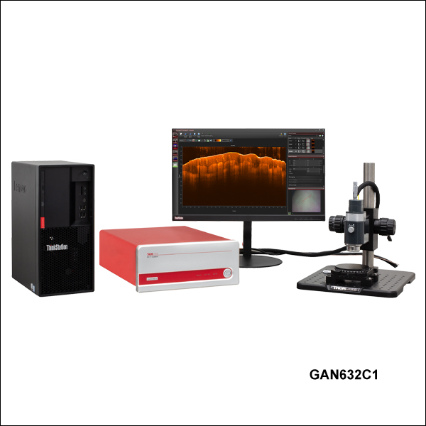
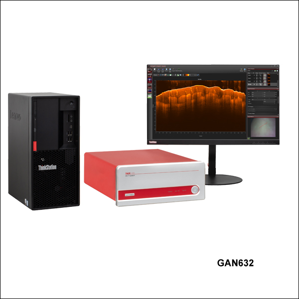
GanymedeシリーズのOCT基本構成システムとして5種類の製品をご用意しております。何れもGanymedeシリーズのすべてのOCTコンポーネントに対応します。GAN111C1/M、GAN312C1/M、およびGAN612C1/Mには880 nmスーパールミネッセントダイオード(SLD)が組み込まれており、高分解能のイメージングが可能です。GAN332C1/MおよびGAN632C1/Mは高分解能を必要とする高速イメージング用として設計されています。3つのスーパールミネッセントダイオードが組み込まれており、それらを組み合わせて880 nmを中心波長とする広帯域光源を構成しています。Ganymedeシステムの最高Aスキャンレートは248 kHz、感度は1.5 kHzで106 dBです。
こちらのGanymedeシリーズOCTシステムは、すべて下記のコンポーネントから構成されています。各システムとも、OCTの3つの中核的なコンポーネント(ベースユニット、走査システムと参照光路長調整用アダプタ、走査レンズキット)、および2つのオプションアクセサリ(スキャナ用スタンド、移動ステージ)から構成されています。基本構成に含まれるコンポーネントについての詳細をご覧になるには、左下の表のリンクをクリックしてください。該当する製品の説明箇所に移動することができます。
システムの詳細やカスタム構成に関するご質問は、当社までお問い合わせください。
| Table G1.1 Preconfigured System Included Componentsa | |||||
|---|---|---|---|---|---|
| System Item # | GAN111C1(/M) | GAN312C1(/M) | GAN332C1(/M) | GAN612C1(/M) | GAN632C1(/M) |
| Base Unit | GAN111 | GAN312 | GAN332 | GAN612 | GAN632 |
| Scanning System | OCTG9 (Standard Scanner) | ||||
| Scan Lens Kit | OCT-LK3-BB | OCT-LK3-BB | OCT-LK2-BB | OCT-LK3-BB | OCT-LK2-BB |
| Reference Length Adapter | OCT-RA3 | OCT-RA3 | OCT-RA2 | OCT-RA3 | OCT-RA2 |
| Accessories: Scanner Stand and Translation Stage | Imperial Systems: OCT-STAND (Stand) and OCT-XYR1 (Stage) Metric Systems: OCT-STAND/M (Stand) and OCT-XYR1/M (Stage) | ||||
| Table G1.2 Preconfigured System Key Specifications | |||||
|---|---|---|---|---|---|
| System Item # | GAN111C1(/M) | GAN312C1(/M) | GAN332C1(/M) | GAN612C1(/M) | GAN632C1(/M) |
| Center Wavelength | 880 nm | ||||
| Imaging Depth (Air/Water) | 3.4 mm / 2.5 mm | 3.4 mm / 2.5 mm | 1.6 mm / 1.2 mm | 3.4 mm / 2.5 mm | 1.6 mm / 1.2 mm |
| Axial Resolution (Air/Water) | 6.0 µm / 4.5 µm | 6.0 µm / 4.5 µm | < 3.0 µm / < 2.2 µm | 6.0 µm / 4.5 µm | <3.0 µm / <2.2 µm |
| Lateral Resolution | 8.0 µm | 8.0 µm | 4.0 µm | 8.0 µm | 4.0 µm |
| A-Scan/Line Rate | 1.5 - 20 kHza | 1.5 - 80 kHzb | 5 - 248 kHzc | ||
| Sensitivity (Max)d | 106 dB (at 1.5 kHz) | 102 dB (at 5 kHz) | |||
")
 ズーム
ズーム OCTシステムの構築にはベースユニットと走査システム、および走査レンズキットが必要です。
| Computer Specificationsa | |||
|---|---|---|---|
| Base Unit Item # | GAN111 | GAN3x2 | GAN6x2 |
| Operating System | Windows® 11 | ||
| Processor | 4 Core, 3.6 GHz | 8 Core, 3.0 GHz | |
| Memory | 16 GB | 32 GB | |
| Hard Drive | 256 GB SSD | 512 GB SSD | |
| Data Acquisition | USB 3.0 | USB 3.0 | CameraLink |
- イメージング速度は柔軟に選択可能、分解能は高分解能または超高分解能から選択可能
- 最高Aスキャンレート:248 kHz(Table G2.1参照)
- より大きな実験装置への組み込みを可能にするトリガ設定
- OCT信号を他のデータソースと結合するためのアナログ入力
- トラブルシューティング機能を改善する内部ハードウェア診断
OCTシステムのイメージング性能は、ベースユニットの設計とそこに組み込まれるコンポーネントに大きく依存します。当社のすべてのOCTベースユニットには、OCTエンジン、高性能PC、プリインストール済みのソフトウェア、およびソフトウェア開発キット(SDK)が含まれています。システムを動作させるには、ベースユニットとあわせて、走査システムと走査レンズキット(いずれも別売り、下記参照)が1種類ずつ必要です。
Ganymede®シリーズのOCTエンジンは、スーパールミネッセントダイオード光源、走査用電子回路、およびリニアCCDアレイをベースにした検出用分光器から構成されています。Ganymedeシリーズのベースユニットに組み込まれたカメラは高速かつ高感度で、そのAスキャンレート1.5 kHz~248 kHz、感度は1.5 kHzで106 dBです。エンジンおよび検出用部品は、411.8 mm x 325.0 mm x 143.0 mmのケースに納められています。
ベースユニットには、他の実験装置と同期ができるようにアナログ入力端子が2つ付いています。これにより、他のデータソースをOCT信号と結合したり、オーバーレイしたりすることができます。OCTベースユニットには、当社のThorImage®OCTソフトウェアで様々にプログラミングできるトリガ設定機能があります。トリガ機能としては、外部信号に応答するための入力用と、トリガ信号を送信するための出力用の両方の動作が可能です。トリガ信号は、Aスキャン、Bスキャンあるいはボリュームスキャンの開始時に送信することも、任意の回数のスキャンを行った後に送信することもできます。
高分解能イメージングベースユニット
ベースユニットGAN111、GAN312、GAN612には、880 nmスーパールミネッセントダイオード(SLD)光源が組み込まれており、空気中において3.4 mmのイメージング深度と6.0 µmの軸方向分解能が得られます。ベースユニットGAN312およびGAN612の最高Aスキャンレートは、それぞれ80 kHzおよび248 kHzです。
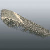
超高分解能イメージング用ベースユニット
超高分解能ベースユニットGAN332およびGAN632は、中心波長880 nmにおいて当社製品の中で最も高いOCTイメージング分解能を有します。3つのスーパールミネッセントダイオード(SLD)を組み合わせた広帯域の光源を使用することで、軸方向分解能として< 3 μm、空気中でのイメージング深度として1.6 mmが得られています。ベースユニットGAN332およびGAN632の最高Aスキャンレートは、それぞれ80 kHzおよび248 kHzです。これらのベースユニットは散乱試料の高分解能イメージングに適しています。
| Table G2.1 Specifications | |||||
|---|---|---|---|---|---|
| Base Unit Item # | GAN111 | GAN312 | GAN332 | GAN612 | GAN632 |
| Description | High Resolution | High Resolution | Very High Resolution | High Resolution | Very High Resolution |
| Center Wavelength | 880 nm | ||||
| Imaging Depth (Air/Water) | 3.4 mm / 2.5 mm | 3.4 mm / 2.5 mm | 1.6 mm / 1.2 mm | 3.4 mm / 2.5 mm | 1.6 mm / 1.2 mm |
| Axial Resolution (Air/Water) | 6.0 µm / 4.5 µm | 6.0 µm / 4.5 µm | < 3.0 µm / < 2.2 µm | 6.0 µm / 4.5 µm | < 3.0 µm / < 2.2 µm |
| A-Scan Line Rate | 1.5, 5, 10, & 20 kHz | 1.5, 5, 10, 20, 40, & 80 kHz | 5, 10, 25, 50, 100, 200, & 248 kHz | ||
| Sensitivitya | 96 dB (at 20 kHz) to 106 dB (at 1.5 kHz) | 89 dB (at 80 kHz) 106 dB (at 1.5 kHz) | 84 dB (at 248 kHz) to 102 dB (at 5 kHz) | ||
| Maximum Pixels per A-Scan | 1024 | ||||
| Compatible Scanners | OCTP-900, OCTP-900/M, and OCTG9 | ||||
Click to Enlarge
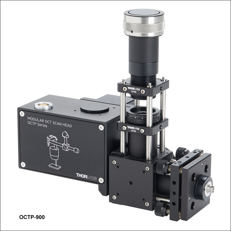
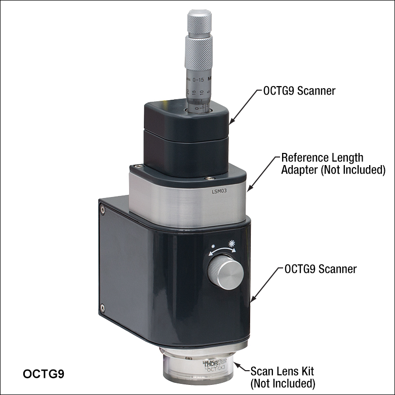
Figure G3.2 調整機能付きOCTスキャナ
Click for Details
Figure G3.1 走査レンズキットと参照光路長調整用アダプタ(いずれも別売り)を取り付けた高剛性(標準型)OCTスキャナ
| Scanner Type | Item # | Compatible Base Units |
|---|---|---|
| Standarda | OCTG9 | GAN111 GAN312 GAN332 GAN612 GAN632 |
| User-Customizable | OCTP-900(/M) |
- OCT光源から試料への照射ビームを走査して2Dまたは3D画像を取得
- 以下の2種類をご用意
- 安定性が高く操作が容易な高剛性(標準型)スキャナ
- 走査光路のカスタマイズが可能なオープン構造の調整機能付きスキャナ
当社のOCT走査システムは、OCT光源からサンプルへの照射ビームを走査させて2次元断層画像または3次元ボリューム画像を取得できるように設計されています。OCTは生体イメージングから工業材料分析まで幅広くお使いいただけますが、それぞれの用途に応じた走査パラメータの設定が必要となります。当社ではGanymede®ベースユニットと一緒にご使用いただく走査システムとして、高剛性スキャナと調整機能付きスキャナをご用意しています。
各スキャナには、サンプルアームならびに参照アームの付いたOCT干渉計が組み込まれています。OCT干渉計の参照アームは試料の近くに配置され、走査システムの筐体内に収納されています。それによりサンプルアームの参照アームに対する位相安定性を維持しています。試料までの距離や反射率が変化すること(例えば、水を通してイメージングする場合など)を考慮して、参照アームの光路長と光強度は調整できるようになっています。分散による画像の歪みを最小化するために、当社のOCTシステムは参照アームとサンプルアームの長さができるだけ光学的に一致するように設計されています。試料による分散の影響(例えば、水やガラスを通したイメージング)は、付属のThorImage®OCTソフトウェアを使用して補正可能です。非共通光路のセットアップをご希望される場合には、いずれのスキャナもビームスプリッタ無しで構成することが可能です。詳細は当社までお問い合わせください。
すべてのスキャナにはカメラが内蔵されており、OCT測定中にThorImage OCTソフトウェアを使用して試料のen face映像をリアルタイムで撮影することができます(詳細は「ソフトウェア」タブをご参照ください)。試料の照明には、各スキャナの出射開口部の周囲にリング状に配置された、調節可能な白色LED光源を使用します。
OCTシステムの構築にはベースユニットと走査システム、および走査レンズキットが必要です。
高剛性(標準型)スキャナ
高剛性スキャナOCTG9は、安定で操作が容易なイメージングシステム用に適しています。高剛性スキャナの筐体は堅牢で遮光性があり、ミスアライメントのリスクを最小限に抑えます。高剛性スキャナ上部には、参照アームの長さの精密な測定と調整を行うためのマイクロメーターネジが付いています。こちらのスキャナには別途参照光路長調整用アダプタをご購入いただく必要があります。
調整機能付きスキャナ
調整機能付きスキャナOCTP-900/Mはオープン構造になっており、当社の標準的なオプトメカニクス部品を使用して光路を簡単にカスタマイズできます。数箇所にSM1ネジ付きポートと#4-40タップ穴が配置されており、それぞれにSM1ネジ付き部品または30 mmケージシステム用部品を取り付けることができます。走査レンズ用ポートにはM25 x 0.75またはSM1ネジ付き部品を直接取り付けられますが、当社のネジアダプタを使用することでRMSのような他のネジ規格にも対応可能です。追加の走査および非走査用光入出射ポートを利用して、蛍光励起用レーザまたは追加の試料用照明を組み込むこともできます。
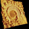
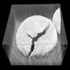
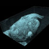
Figure G4.1とG4.2のリンゴの画像は、Ganymede®シリーズのOCTシステムに走査レンズキットOCT-LK2-BBおよびOCT-LK3-BBを取り付けて取得したものです。 走査レンズキットは、用途に合った解像度、焦点距離のものをお選びください。

- テレセントリック走査レンズによるフラットな結像面
- 800~1100 nm対応のARコーティング付きレンズ
- 高剛性/調整機能付きスキャナ用の走査レンズキットには以下のものが含まれます。
- テレセントリック走査レンズ
- 照明用チューブ
- 赤外域ビュワーカード
- 校正用ターゲット
- 分散補償用セット
 OCTシステムとして動作させるには、ベースユニット、走査システム、走査レンズキットが必要となります。
走査レンズキットにより、OCTシステムの走査レンズを簡単に交換できるため、イメージングの分解能や作動距離を用途に合わせて様々に設定することができます。 こちらのレンズキットは、OCT用テレセントリック走査レンズをベースとしているため、測定後の画像処理を用いずとも像の歪みを最小限化し、同時に試料から散乱または発する光を検出システムに最大限結合させます。Table G4.3のように、当社では高剛性スキャナ(型番 OCTG9)用および調整機能付きスキャナ(型番 OCTP-900/M)用のレンズキットを3種類ご用意しています。
各キットにはテレセントリック走査レンズ、照明用チューブ、赤外域ビュワーカード、校正用ターゲットが付属します。 照明用チューブはライトガイドとしてLED照明リングからの光を試料の領域に伝送します。赤外域ビュワーカードならびに校正用ターゲットを用いて走査ミラーおよびレンズキットの校正を行い、走査レンズを交換しても良好な画質を得られるようにします。
| Table G4.3 Specifications | |||
|---|---|---|---|
| Scan Lens Kit Item # | OCT-LK2-BB | OCT-LK3-BB | OCT-LK4-BB |
| Click Image to Enlarge | 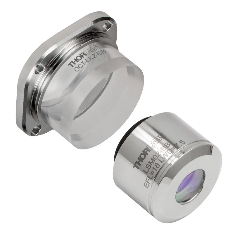 |  |  |
| Design Wavelength | 880 nm / 900 nm / 930 nm / 1060 nm | ||
| Compatible Scanner | OCTG9 (Standard) or OCTP-900(/M) (User-Customizable) | ||
| Lateral Resolutiona | 4 µm | 8 µm | 12 µm |
| Effective Focal Length | 18 mm | 36 mm | 54 mm |
| Working Distance | 3.4 mm (with Tube)b 7.5 mm (without Tube) | 24.9 mm (with Tube)b 25.1 mm (without Tube) | 41.6 mm (with Tube)b 42.3 mm (without Tube) |
| Field of View | 6 mm x 6 mm | 10 mm x 10 mm | 16 mm x 16 mm |
| Lens Threading | M25 x 0.75 | M25 x 0.75 | M25 x 0.75 |
")
 ズーム
ズーム| Table G5.1 Specifications | |
|---|---|
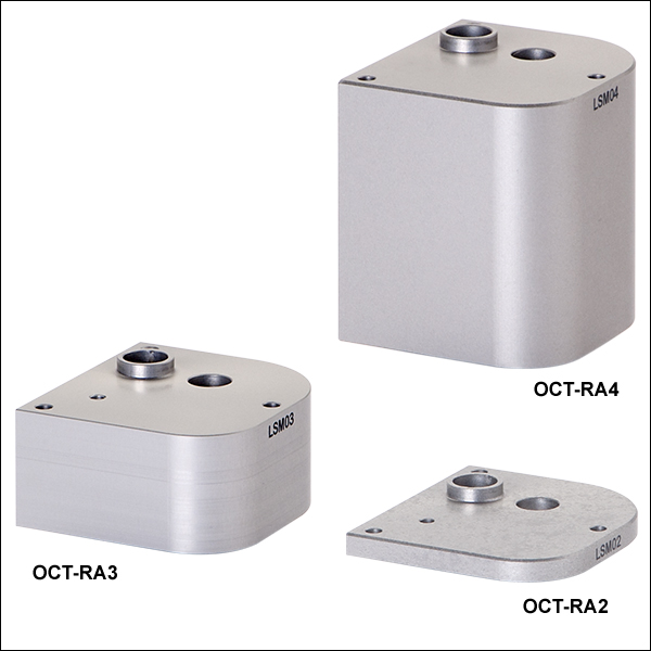
| Item #a | Compatible Scan Lens Kit |
| OCT-RA2 | OCT-LK2-BB |
| OCT-RA3 | OCT-LK3-BB |
| OCT-RA4 | OCT-LK4-BB |
- 参照光路長とサンプル光路長を一致させるためのアームアダプタ
- 複数のアダプタの使用で走査レンズキットの素早い交換が可能
- 高剛性スキャナ(型番 OCTG9)には必須
こちらのアダプタを使用して高剛性スキャナOCTG9内の参照アーム光路長を調整し、使用した走査レンズにより違うサンプル光路長に一致させることができます。3種類の中から上記掲載の走査レンズキットに対応する製品をお選びください。参照光路長調整用アダプタにより、走査レンズキットを再調整せずに素早く交換することができます。適切なアダプタを選択する際の対応表をTable G5.1に掲載しています。
")
- 試料からの最適な作動距離にスキャナを設置
- リング型(空気用)および液浸型(液体用)のZスペーサをご用意
当社では、走査システムと試料間の距離を最適に設定するための、リング型、液浸型の両タイプの試料用Zスペーサをご用意しています。ZスペーサOCT-AIR3、OCT-IMM3およびOCT-IMM4は、刻み付きリングで間隔距離の調整を行います。安定性を向上させるため、適切な位置にリングをロックすることができます。Zスペーサは数種類の中からお選びいただけます。Table G6.1のスキャナおよびレンズキットとの対応表をご参照ください。
リング型Zスペーサは、スキャナと試料間のディスタンスガイドとなります。試料はスペーサのリング状の先端に接触させます。このスペーサは、空気を走査媒体とする場合のみご使用いただけます。これに対し、液浸型スペーサにはガラス板が付いており、走査領域内で試料表面に接触させます。リング型スペーサとは異なり、液浸型スペーサは液体内の試料の安定性を保ったまま試料にアクセスできます。屈折率整合した傾斜付きのガラス板を使用することで、試料表面からの強い後方反射を減少させ、画像のコントラストを向上させることができます。
| Table G6.1 Specifications | ||||||
|---|---|---|---|---|---|---|
| Item # | Type | Adjustable | Adjustment Range | Lockable | Compatible Scanner | Compatible Scan Lens Kit |
| OCT-AIR3 | Ring (Air) | Yes | +3.5 mm / -1.0 mm | Yes | OCTG9 OCTP-900(/M) | OCT-LK3-BB |
| OCT-IMM3 | Immersion | Yes | +3.4 mm / -1.1 mm | Yes | ||
| OCT-IMM4 | Immersion | Yes | +1.0 mm / -17.0 mm | Yes | OCT-LK4-BB | |
")
 ズーム
ズーム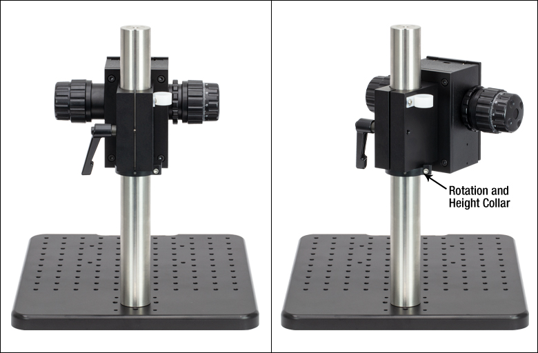
Click for Details
Figure G7.1 集光ブロックは45°回転可能で、スキャナーヘッドを試料から離すことができます。
- 高剛性または調節機能付きスキャナ取付け用の推奨スタンド
- Ø38 mm(Ø1.5インチ)ステンレススチールポストに取り付けたZ軸粗微動可能な集光ブロック
- M6タップ穴付きの300 mm x 350 mmアルミニウム製ブレッドボード
血管造影のような振動に敏感な研究に適した、高剛性または調整機能付きスキャナを取り付けしやすいスタンドです。ポストに取付け済みの集光ブロックは、ノブでZ軸粗動(40 mm/回転)および微動(225 µm/回転)調整が可能です。 集光ブロックの下にある回転および高さ調整カラーにより45°回転し、スキャナーヘッドを試料から離して調整を行うことができます。
集光ブロックは付属のØ38 mm(Ø1.5インチ)ポストを介して300 mm x 350 mmのアルミニウム製ブレッドボードに取り付けられています。このブレッドボードにはサイドグリップとゴム製の脚がついており、簡単に持ち運びできます。オプトメカニクスを取り付けるためにM6タップ穴の配列があります。また移動ステージOCT-XYR1/M(下記掲載)をOCT-STAND/Mの走査レンズの真下に直接設置するためのM6取付け穴が4つと、Ø38 mm(Ø1.5インチ)ポストを固定するためのM6ザグリ穴が1つ付いています。
")
 ズーム
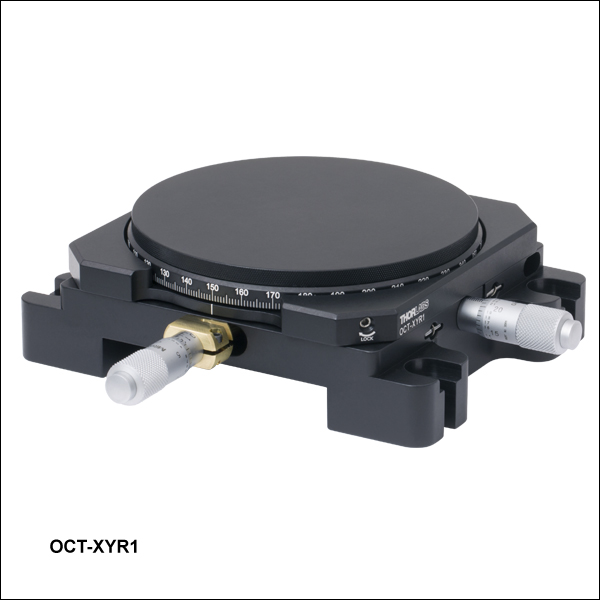
ズームClick to Enlarge
Figure G8.1 カバープレートを取り外してタップ穴およびSM1ネジ付きの中心穴にアクセスできます。
| Specifications | |
|---|---|
| Horizontal Load Capacity (Max) | 10 lbs (4.5 kg) |
| Mounting Platform Dimensions | Ø4.18" (Ø106 mm) |
| Stage Height | 1.65" (41.8 mm) |
| Linear Translation Range | 1/2" (13 mm) |
| Travel per Revolution | 0.025" (0.5 mm) |
| Graduation | 0.001" (10 µm) per Division |
- 13 mmのXY移動ならびに360°回転が可能なオプションの移動ステージ
- 試料を取り付けるためのカバープレート付き
- カバープレートを取り外してオプトメカニクスを取付け可能
OCTイメージングの準備中ならびに実行中に試料の位置決めを正確に行うためには、精密移動および回転が必要となります。OCT-XYR1/MにはXY直線移動ステージに加え、回転式プラットフォームとクリーニングしやすい試料固定用剛性カバープレートを搭載しています。 OCT-XYR1/Mは、4隅にあるM6ザグリ穴を使用して上記掲載のOCT-STAND/Mに固定することができます。上部プレートを取り外して#4-40、M4、およびM6タップ穴、ならびにSM1ネジ付き中心穴にアクセスし、オプトメカニクス部品が取り付け可能です。試料用プレートXYR1Aには穴が無く、上面プレートの代わりとして別途ご購入いただけます。
X軸とY軸のマイクロメータの移動量は13 mmで、10 µm刻みの目盛が付いています。 ステージは、取り付けた部品の安定性を損なうことなく自由に回転・移動させることができます。回転式プラットフォームの外端に沿って刻まれている角度目盛により、ステージの角度を設定してからロック用止めネジ(2 mmの六角穴付き)で固定することができます。回転を固定しても、アクチュエータを用いてXY軸での移動は可能です。